Biostatistical Significance and Confidence Intervals in Public Health

Research updated on August 6, 2025
Author: Santhosh Ramaraj

In biostatistics, answers are rarely a simple yes or no. Instead, researchers interpret results based on a measure called statistical significance. This is most often expressed as a p-value, which tells you the probability of obtaining your observed result, or something more extreme, if the null hypothesis were actually true. A smaller p-value means the result is less likely to have happened purely by chance.

However, statistical significance does not always mean the result has practical importance. In a large drug trial, a medication might show a statistically significant reduction in symptom scores, yet the effect could be so small that patients would hardly notice it. This gap between mathematical and practical meaning is something every public health professional must keep in mind.

Statistical Significance vs Practical Relevance

A finding can be statistically significant yet clinically unimportant.

Imagine a study involving 50,000 participants where a new nutrition program reduces average weight by 0.2 kilograms. With such a large sample size, the p-value may be extremely small, leading you to reject the null hypothesis. But in real-world terms, a 0.2 kilogram change might not be meaningful for improving community health.

This is why public health professionals should always interpret p-values alongside other measures such as effect size, risk difference, and confidence intervals.

Variation in Public Health Measurements

Public health data often come from surveys, registries, or surveillance systems. While these datasets can estimate the prevalence of health issues, they are not always perfect reflections of the true underlying risk in the population.

Two main factors cause this variation:

Sampling error — differences between the sample estimate and the true population value simply because only part of the population is measured.
Random variation — differences that occur even if the entire population is measured, due to chance events in real life.

What is Sampling Error?

Sampling error is the random variation you get when measuring only part of the population. Even if the sampling process is done correctly, results from one sample will differ from another.

For example:

In a survey of 1,000 households, 14 percent report having no access to clean drinking water.
In a different random sample of 1,000 households from the same community, 15 percent may report the same problem.

This difference is not necessarily due to changes in the community, but simply the randomness of which households were selected. Sampling error decreases when the sample size increases, which is why large studies tend to give more precise estimates.

Random Variation Even in Full Counts

Even when you measure an entire population, random variation still exists. For example, the number of heart attacks in a city this year might be 1,200, while last year it was 1,150. This difference could occur purely by chance, even if the underlying risk in the population has not changed.

In statistical terms, both of these counts are just one of many possible outcomes that could occur under the same circumstances.

Confidence Intervals. Measuring Precision

A confidence interval (CI) is a range of values that likely contains the true population value. It reflects the uncertainty in your estimate.

A 95% CI means that if you were to take an infinite number of samples of the same size from the same population and calculate a CI for each sample, about 95% of those intervals would include the true value.

It is important to understand that the CI does not mean there is a 95% probability that the true value is inside the interval for your one study. The interval is fixed once calculated, and the 95% refers to the performance of the method over repeated sampling.

Why Confidence Intervals Are Important

Confidence intervals add context to p-values. Two studies may have identical p-values, but the width of the CI tells you whether the estimate is precise or uncertain.

Example:

Study A: 10 percent obesity prevalence, 95% CI 9 to 11 percent.
Study B: 10 percent obesity prevalence, 95% CI 5 to 15 percent.

Both show the same central estimate, but the first study has much more precision, giving greater confidence in the result.

Calculating the 95% CI for a Percentage

When your data is from a survey and you want to calculate a CI for a percentage, the first step is finding the standard error (SE). In a simple random sample, the formula for the SE of a proportion is:

$SE = \sqrt{\frac{p \cdot q}{n}}$

Where:

= the proportion in decimal form (for example, 40% → 0.40)
= 1 − p (the proportion of the population not in the category of interest)
= the sample size

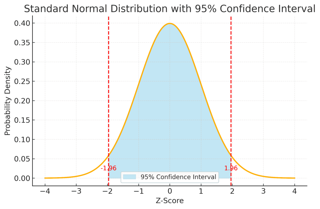
This diagram shows the standard normal distribution, the familiar bell-shaped curve, with the 95% confidence interval shaded in light blue.

Here’s what each part represents:

1. The Horizontal Axis (Z-Score)

The z-score measures how far a value is from the mean in terms of standard deviations.
The center of the graph (z = 0) represents the mean of the distribution.
Negative z-scores are values below the mean, positive z-scores are above the mean.

2. The Bell Curve

The curve shows the probability density of the standard normal distribution, which has a mean of 0 and a standard deviation of 1.
Most of the values are clustered near the mean, and the curve tapers off as you move further away.

3. The Shaded Blue Area (95% Confidence Interval)

The shaded region covers z-scores from -1.96 to +1.96.
This range contains approximately 95% of the total area under the curve.
In statistical terms, if we repeatedly took random samples and calculated estimates, 95% of those estimates would fall within this range around the true mean.

4. The Vertical Red Dashed Lines

These lines mark z = -1.96 and z = +1.96, which are the cut-off points for the 95% confidence interval.
The small unshaded tails on each end (2.5% each) represent the extreme values that fall outside the 95% range, these are more unusual outcomes.

5. How to Interpret

If your calculated statistic (converted to a z-score) falls inside the shaded area, it means it is within the expected range for 95% of random samples.
If it falls outside, it is considered statistically unusual, and you might reject the null hypothesis (assuming your significance level is 5%).

Worked Example 1

A survey of 1,000 adults finds that 40 percent exercise at least three times per week.

Step 1: Calculate
$q = 1 - p = 1 - 0.40 = 0.60$

Step 2: Calculate the SE
$SE = \sqrt{\frac{0.40 \times 0.60}{1000}}$
$SE = \sqrt{\frac{0.24}{1000}}$
$SE = \sqrt{0.00024}$
$SE \approx 0.01549$

Step 3: Find the margin of error for a 95% CI using $z = 1.96$
$ME = 1.96 \times 0.01549 \approx 0.03036$

Step 4: Apply the margin of error to $p$
$CI = 0.40 \pm 0.03036$

Result: 37.96 percent to 43.04 percent

Worked Example 2

A community health survey of 400 children finds that 18 percent are underweight.

Step 1: , so
$q = 1 - 0.18 = 0.82$

Step 2:
$SE = \sqrt{\frac{0.18 \times 0.82}{400}}$
$SE = \sqrt{\frac{0.1476}{400}}$
$SE = \sqrt{0.000369}$
$SE \approx 0.01921$

Step 3:
$ME = 1.96 \times 0.01921 \approx 0.03763$

Step 4:
$CI = 0.18 \pm 0.03763$

Result: 14.24 percent to 21.76 percent

The Role of the Normal Distribution

The idea of the CI is tied to the normal distribution. Many statistics, such as averages, proportions, and rates, follow a distribution that becomes approximately normal when the sample size is large enough.

A z-score tells you how far a value is from the mean in terms of standard deviations.

For a 95% CI, the z-score is 1.96, which leaves 2.5% of the distribution on each side.
For a 90% CI, the z-score is 1.65, leaving 5% on each side.

This is why multiplying the SE by 1.96 gives the margin of error for a 95% CI.

Common Pitfalls in Interpreting CIs

Confusing statistical significance with importance: A narrow CI around a tiny effect may still have little real-world value.
Over-relying on the central estimate: The true value could be anywhere in the interval.
Ignoring the sample size: Wide intervals often come from small samples and should be treated with caution.
Misunderstanding the 95%: It is not the probability that the true value is in your interval; it is about the method’s accuracy over repeated sampling.

Putting It Into Practice

If your vaccination coverage survey shows 92 percent coverage with a 95% CI from 91 to 93 percent, you can be confident the true rate is close to your estimate. But if the CI is 85 to 99 percent, more data collection or a larger sample may be needed before deciding whether targets are met.

Confidence intervals, combined with knowledge of sampling error, help to interpret findings realistically and make better policy decisions.

Relevant Reads